You Can Still Find Mispriced Options in 2026

The unglamorous but profitable business of pricing your own options.

“There’s no edge in vanilla options anymore. The surfaces are too clean, the market makers are too good, and you’re not finding anything in 2026 that a desk in Chicago didn’t price five minutes ago.”

If you spend any time around trading discourse, you’ve likely heard some version of this take. It’s confidently delivered, usually by someone who once tried selling weekly strangles and got tagged.

And to be fair, it’s not totally wrong.

SPX options in 2026 really are as close to efficient as it gets. The days of catching obvious mispricings on a Bloomberg terminal at lunch are over, and they have been for a while.

What gets lost in this take though, is that “mispriced” was always the wrong word for it.

At the end of the day, professional options trading isn’t about hunting quotes that are wrong against some objective truth, but rather about taking the public price, comparing it to your own internal price, and putting on a trade if the difference is big enough.

So, it’s less “this option is objectively priced wrong” and more “this option is cheap/rich relative to this specific assumption”.

Unfortunately however, the whole process of pricing your own options around a bespoke view is extremely vague if not totally inaccessible to most non-MM traders.

So today, we want to crack-open that process and show you first-hand how you can intuitively use sophisticated options models to not just price options “better” than what you see on screen, but also how you generate some of these views and assumptions to begin with.

Without further ado, let’s get right into it.

It Goes Way Deeper Than Black-Scholes

To begin, we have to understand why anyone even bothers to use anything other than Black-Scholes in the first place.

An option model, at root, is a story about how the underlying behaves between now and expiration.

Black-Scholes tells the clean version where markets are basically random walks and implied vol tends to stay the same throughout its life.

As a description of how markets actually behave, though, it’s not really true:

• What about stocks with a momentum factor, where the forward returns are more predictable than just a random walk?

• What about those currently undergoing extreme realized volatility, where implied vol is either way too high or way too low?

So, over the last fifty years the industry has constantly innovated to create new models that better reflect reality in ways the textbook Black-Scholes doesn’t.

To see why this matters, here’s the same 90-day 105-strike put on a $100 underlying, priced under five different models with identical observable inputs (5% rate, no dividends, 25% vol):

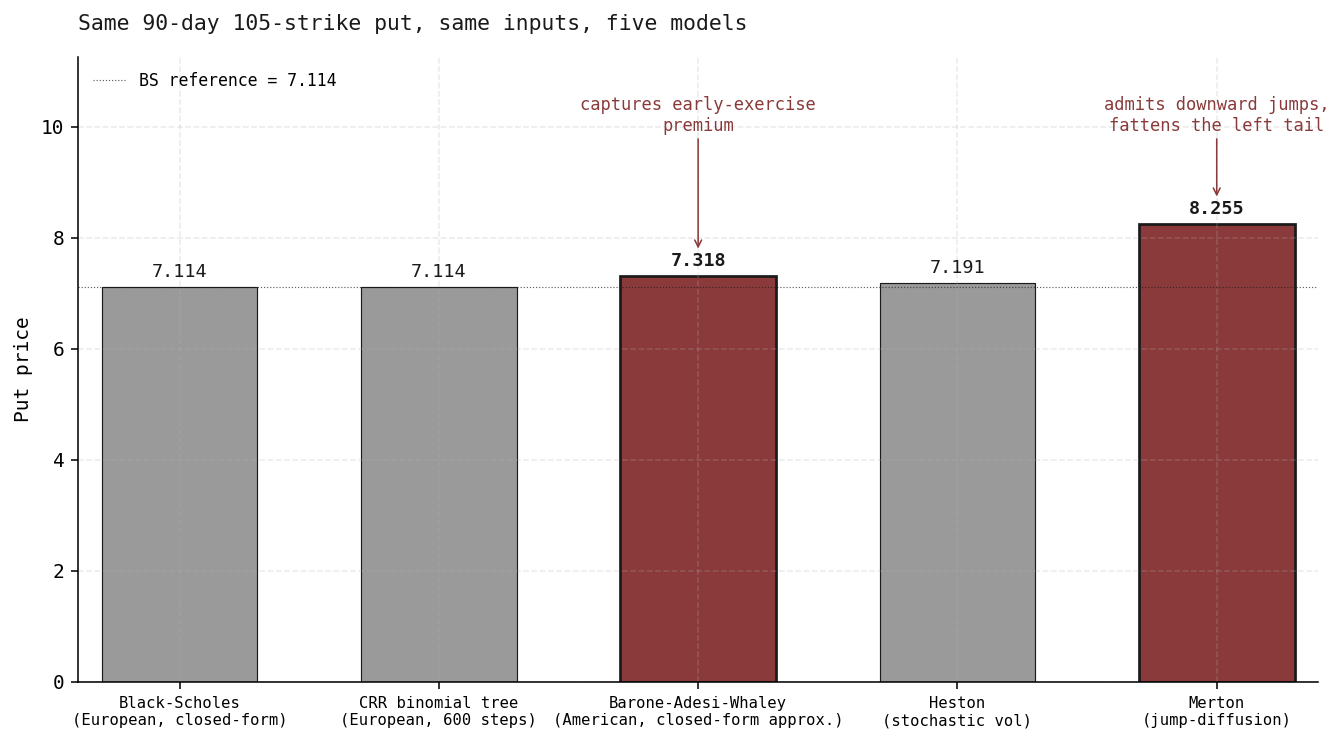
Two commonly used industry models, Barone-Adesi-Whaley and Merton Jump-Diffusion, are demonstrable standouts compared to the typical Black-Scholes price, and for a good reason:

• Barone-Adesi-Whaley model

  • Put simply, this is the Black-Scholes model, but with a small premium to cover the early-exercise risk in American Options.

    • SPX and index options can use BS since they’re cash-settled and have no early exercise risk, but single stock options have the added risk of being able to be exercised for shares at any time.

• Jump-Diffusion model

  • In sum, this model is used when prices trade discontinuously rather than in a smooth drift like assumed in Black-Scholes. The left-tail risk is also priced higher, so OTM options carry a higher than average premium.

    • If there is an upcoming event (earnings, regulatory ruling, etc.), the price can have 1 day where it abruptly goes in either direction, so this model comes in handy.

So, right off the bat, in professional options trading, the model used is often very case-dependent.

When pricing American options, you might use the BAW model, but when pricing those options knowing that a huge event is on the horizon, you might layer on a Jump-Diffusion model.

Now, this might still seem a bit theoretical, so to really cement the understanding, let’s walk through an actual trading example.

How Do You Make Money With This Stuff?

Okay, it’s Wednesday at 12:00 PM and we’re discretionary vol traders looking for cheap options.

First, we need a name.

Scrolling through a screener, we land on CVNA.

A high-quality short report dropped on it three days ago, we've read the report, we think most of it is fair, and we're roughly aligned with the thesis. The stock is down about 2% on the week and volume is unremarkable.

The options market is pricing things like nothing happened.

That last part is the trade.

The short report is sitting in plain view, and either the market digests it over the next quarter and the stock leaks lower, or the next earnings call poses a tough enough question that the bid evaporates faster than that.

Either way, we think realized vol on a 6-month horizon is going to come in higher than the surface is pricing.

The cleanest way to express this without taking a directional view is the 6-month at-the-money straddle. We don’t need to be right about which way; we just need to be right that something happens.

So, we pull up our Options Pricer, select the Merton jump-diffusion model (we think a large sudden move is likely), and input the metrics as it’s trading now:

Access the Alphanume options pricer, plus bond and futures pricing tools, at alphanume.com.

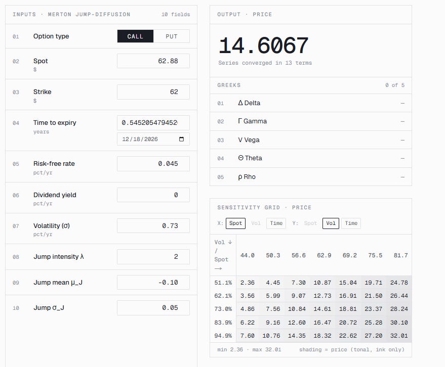
Quick clarification on some terms:

• Jump intensity λ: how often jumps happen, in jumps per year on average. λ = 2 means we expect two material discontinuous moves per year, on average. Higher λ means jumps are more frequent.

• Jump mean μ_J: the average size of a jump given that one occurs, expressed in log terms (so roughly a percentage move). μ_J = −0.10 means jumps tend to be downward, around −10% on average. A symmetric view would set μ_J = 0; an upside-biased name (think a biotech awaiting an FDA decision) might set it positive.

• Jump dispersion σ_J: how much variation there is around that mean jump size. σ_J = 0.20 means that when a jump happens, it’s not always exactly −10%; it could be −5% or −25% or +5%, with the spread around the mean governed by this parameter. Larger σ_J means jumps are more variable in magnitude.

So, right off the bat, our fair view of that 6-month call option is a price of ~$14.60.

Now, we check what the option is currently trading at on the open market:

Midpoint of ~$14.15

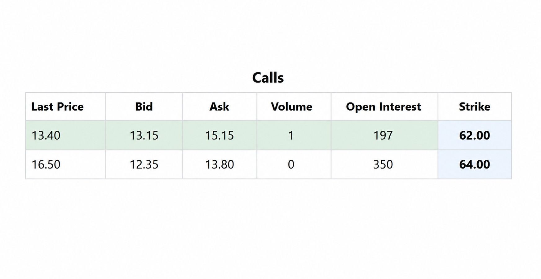
At the time of capture, the 6-month call was trading at around $14.15 against our fair value of $14.60. Not a marked difference, and on its own, not enough to put on a trade.

But there’s a major caveat before we stop here.