

At root, selling options is a pretty simple deal:
Market participants pay premiums for contracts tied to unlikely events
You sell them those contracts and collect said premiums
Once in a while, the event actually happens, and you have to pay back some premiums
Repeat
Where things get tricky is when you realize that everyone else is also aware of this, and thus the contracts are pretty close to efficient.
For instance, if you’re offered a spread with a 95% implied probability of expiring worthless, it will do that ~95% of the time.
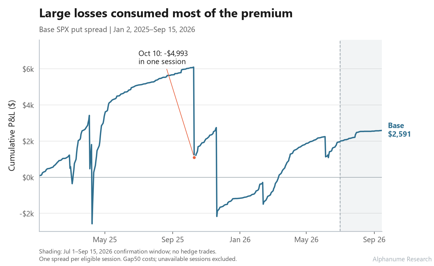
Stats 101 tells us that such an offering results in 0 EV, so even if you derive an approach that makes money the majority of the time, your equity curve will generally look like this:
Fortunately though, it doesn’t have to be this way.
Remember, selling options is essentially underwriting insurance. Insurers write out the policy, but more importantly, they constantly buy re-insurance, specifically to prevent the “pennies in front of a steamroller” problem.
So today, we’re going to walk you through what it actually takes to systematically trade these in a +EV fashion. You’ll get a real-world look at effective hedging and by the end, you’ll see why calling these -EV or even efficient is far from reality.
Without further ado, let’s get right into it.
Just hedge, man.
When one is first presented with this reality, the most tempting choice is to try moving around the risk-reward slider.
In practice (and this may look familiar), it generally goes like this:
Your max loss on a short put credit spread is, say, $1,000
To minimize this worst-case loss, you try:
Simultaneously buying the equivalent put spread of a later expiration
Selling a tighter butterfly spread around the at-risk strikes
Buying a deeper OTM put to act as a tail-risk hedge
Each time, as you may already know, the EV still nets out to 0.
This is largely because you’re trying to hedge an already efficiently-priced option position with more efficiently-priced options, so the EV isn’t really coming from anywhere new.
The solution to this is, surprisingly, simply using the underlying.
Now, the appeal of hedging with the underlying is pretty clear (predictable PnL, no views on vol), but to really understand where we’re going, it’ll help to walk through an example.
To start, let’s go back to October 10th last year, which was the single worst day in our test. Here’s how it went for a plain put spread with no hedge:
At 10:30 ET, SPX was at 6750.50, so we sold the 6645 put (about 1.5% below spot) and bought the 6595 put 50 points under it.
The credit came to $8.75, or $6.75 after fees.
SPX sold off all afternoon and closed around 6552, below both strikes, so the spread took its full loss of about $5,000.
The average winner in this test made ~$66, so that one afternoon handed back roughly 75 winning days.
Now, let’s replay the same session with one extra parameter, where the moment SPX touches our short strike, we short SPY shares against the spread:
SPX touched 6645, and after a 1-minute lag for realism, we shorted 409 SPY shares at $662.93
SPY kept falling, and we covered just before the close at $653.25.
The short made about $3,950 after costs, which took the day from a ~$5,000 loss down to about $1,040.
This recovered about 79% of the loss, which should help you see the appeal of this direction pretty quickly.
Of course, we know better than to cherry-pick over 1 trading day, so now that we have a starting framework, we can ask a new question:
What happens when you run this hedge every single day, for years?
The experiment
To find out, I kept the base trade as crude as possible, so any change in the curve comes from the hedge:
Take the 10:30 ET SPX price and find the highest same-day put strike at least 1.5% below spot.
Sell that put and buy the put 50 points lower, using the 10:31 quotes.
Although basic automated scripts are substantially faster, adding in time-lags gives us a realistic basis.
We’ll model giving up half the distance between the mid and the worse side of the quote, as opposed to just assuming a fill at the mid.
We also assume a standard retail brokerage commissions fee of $1 per contract.
Skip the day if the quotes are unavailable or the credit is under 0.05 points (i.e., <$5).
Hold through expiration, using one spread per session with no compounding.
So with the simple baseline strategy established, we can move into how we’ll run the hedging side:
Starting at 10:31, pull each completed SPX one-minute aggregated price.
We stop checking for new triggers at ~2:00 PM ET
On the first bar whose low touches the short strike, short SPY at the next minute’s open.
Size the short at 0.25x, 0.5x, or 1.0x of the spread’s delta at that moment, converted into SPY shares (we’ll explain more on this below).
Keep the share count fixed and cover at EOD.
We’re deliberately not continuously hedging throughout the session to ensure practicality.
Now, step 3, calculating the net delta and converting it into the optimal hedge size, is the most important part, so we can slow down a bit there.
The spread’s delta tells us how many dollars we lose for each point SPX falls, and once we know that, we just short enough SPY to make the same amount back.
Taking the same session replay from above, here’s how that worked:
Derive the implied move of the session
At 10:31, the ATM straddle (6750 call + 6750 put) was pricing about a 22.7-point move for the rest of the day.
Scale the implied move to the remaining time in the session
Expected moves scale with the square root of time, and 273 of the original 328 minutes were left (triggered at ~11:26), so
22.7 × √(273/328)gives us about 20.7 points.
Convert that into implied odds for each strike
We measure how far each strike is in “expected moves”, where a bell curve tells us how often SPX finishes beyond it.
A strike sitting right at the current price is a coin flip (50%), one full expected move away is about 16%, and two is about 2%.
At 11:26, SPX was at 6649.60, just 4.6 points above our 6645 short put. Running
4.6 ÷ 20.7gives about 0.2 expected moves away, which is roughly a 41% chance of finishing below it.The 6595 long put was 55 points away, or
55 ÷ 20.7= 2.6 expected moves, which works out to about 0.4%.If you want to check these yourself, it’s
=NORM.S.DIST(-0.22, TRUE)and=NORM.S.DIST(-2.64, TRUE)in Excel or Sheets.
Subtract the two to estimate the spread’s delta
So,
0.412 − 0.004, or about 0.408, and with the $100 multiplier, the spread was losing about $40.80 for every point SPX dropped.
Convert SPX points into SPY shares
SPX was trading at about 10.03x the price of SPY, so a 1-point SPX move is only about a $0.10 move in SPY. To make $40.80 back per SPX point, we need
40.8 × 10.03, which is the 409 shares from earlier.
Put together, the model is shares = ratio × 100 × spread delta × SPX/SPY, where the ratio is our 0.25x, 0.5x, or 1.0x.
Okay, that was a lot of information at once, so I’d take a second before we move into the PnL.
C’mon, does it work, or not?
Putting it all together, we went back as far as our cached quote data allowed us to, and re-ran the above schematic every single day.
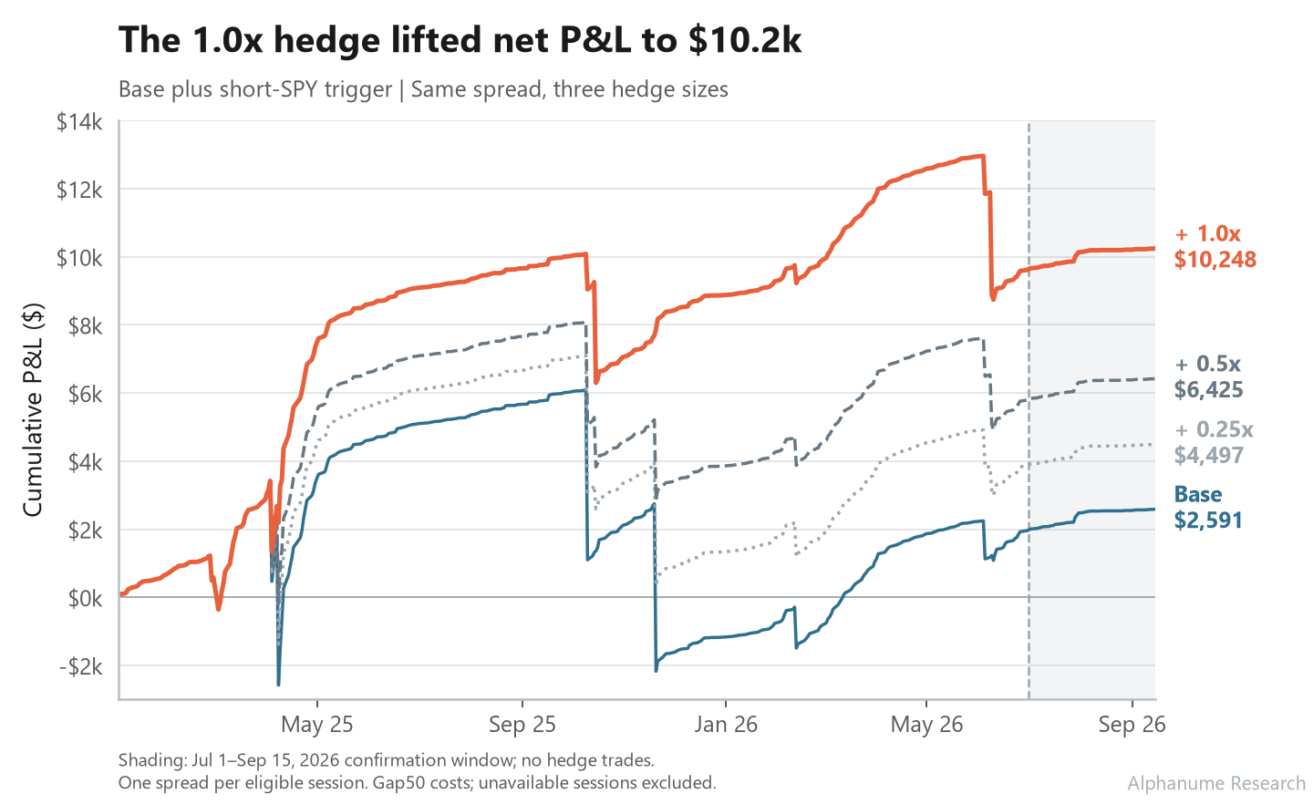
Fortunately, this approach manufactured positive expected value in every single variation:
The big picture results:
Net P&L nearly quadrupled, going from about $2.6k unhedged to $10.2k with the full-size hedge
The largest drawdown fell by about half, from $8.3k down to $4.2k
The worst single day improved by about 40%, from a ~$5k loss to a ~$3k loss
The hedge paid off when it was actually needed
On the nine losing days, the short recovered $14.5k of the $21.4k, roughly 68%
So, although the hedge only fired on a handful of days, it made more on the selloffs than it cost us everywhere else, and we kept far more of the premium while still having something in place for the worst-case sessions.
As usual though, there’s a bit of nuance to this.
Nuanceville
The first thing to know is that, obviously, the hedge often loses money on a day the spread ends up totally fine.
To see this, let’s pull out a session from the run:
SPX touched our short strike, so we shorted 520 SPY shares at ~$659
The market rose right after and we covered near the close at ~$665, for a loss of about $3,000
The spread expired worthless and made $47
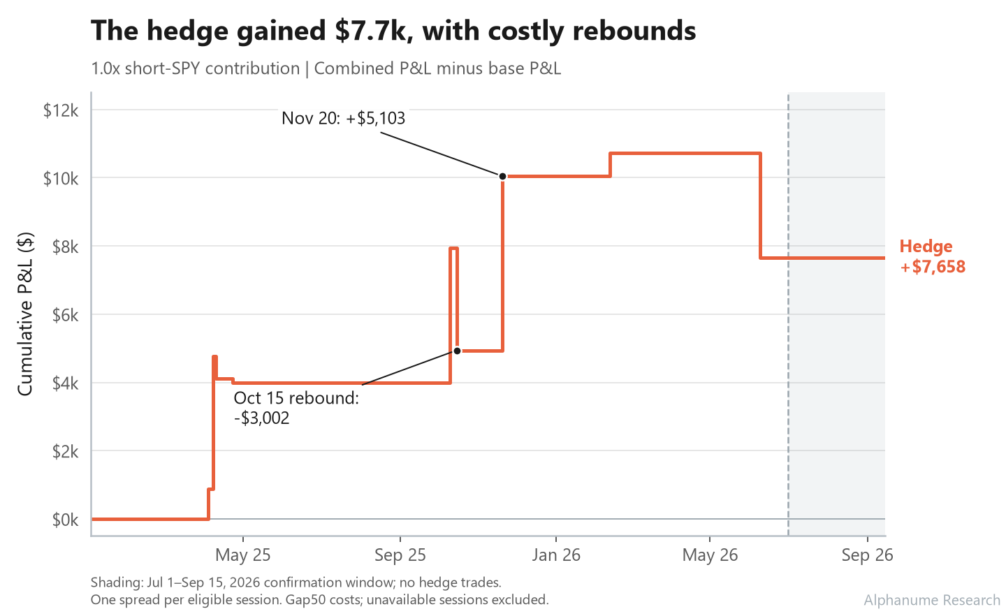
So, even though we only hedge on a trigger, there’s still a cost to hedging. The hedge fired nine times in the whole test, and went like this:
5 triggered on days the spread actually lost, and all 5 made money ($14.5k).
4 triggered on days the spread finished fine, and all 4 lost money (-$6.8k).
Interestingly though, we found that the hedge made money as its own trade.
Net of the rebounds, the short was up about $7.7k by itself (chart below), which suggests that SPX touching the short strike is a bit of a signal in its own right, since the selling continued more often than it reversed.
Lastly, if you haven’t already noticed, this is a pretty capital-intensive trade.
The short in our earlier example was about $271k of SPY against a single spread, and you’d need that much in buying power to hedge on a minute’s notice.
Fortunately, the same framework carries over to futures, as it’s virtually what index futures were made for.
Our spread was losing about $41 per SPX point at the trigger, and a Micro E-mini (MES) contract moves $5 per point, so shorting 8 MES contracts covers roughly the same exposure for a fraction of the capital, with no shares to borrow. We’ll go deeper on that version in a later post (we’re still cleaning the messy futures data - rolls, margin changes, etc.).
Final Thoughts
When 0-DTEs first launched back in 2022, I immediately saw the potential economic value:
Same-day settlement
Deep liquidity
Clear hedgeability
It unfortunately took me too long to get serious about implementing the hedging frameworks that are commonplace at larger option desks.
Our next research direction from here is seeing what the low-cost futures version of this looks like. First though, we opened a can of worms when we first reverse-engineered retail trading patterns in 0-DTE, which led us to some very interesting findings in the single-stock space.
We’re running that new framework live for a few weeks to make sure our code is right, so it’ll take some time to accumulate enough live data to present any findings.
Nevertheless, we hope that if you’re running into the “pennies in front of a steamroller” problem, reading this will have at least given you a real direction on what it takes to fix it.
One more thing before you go.
Everything we publish here starts with a dataset, and those datasets are what we build over at Alphanume. We know better than to ask you to take our word that they’re predictive, so we tested each one against real prices and put the results on our proof page:
IV/HV Premium: the richest 20% of names had implied vol 5.7 points richer than realized, while the cheapest 20% came in 8.7 points below (t = 14.3).
In other words, you can reliably find stocks with cheap vol and expensive vol.
Pre-Market Drop Risk: names that the model marked with 70 % or higher risk averaged a decline of 8.3 % from open to close and 76 % of those names closed lower.
In other words, each day, the dataset reliably publishes those that’re likeliest to fall significantly intraday
Those are just 2 of the simplest examples, but we have 25+ more and we’re adding datasets constantly. If you want to run your own version of experiments like this one, it’s just one API call away.
As always, thanks for reading, and we’ll see you in the next one.